binomial logistic regression

binomial logistic regression models the probability of an observation falling into one of two categories, based on 1 or more independent variables.

Graphically, it looks like an S-shaped logistic function. The model outputs values 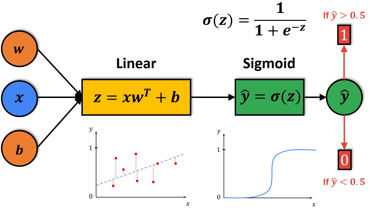between 0 and 1 (a probability)

where is the predicted value. If is large, the predicted probability is close to 1, resulting in the model predicting label 1 for this specific example

Why the name "regression"?

If we rewrite sigmoid function into log-odds

then logit has the form of regression

Assumptions

• Linearity: there should be a linear relationship between each X variable and the logit of the probability that Y equals 1.
• Independent observations
• Little to no multicollinearity
• No extreme outliers

Interpretation

A model classifies obesity at mice, with

• If , there’s 70% chance that the mouse is obese. We classify it as “obese”
• If , there’s only 30% chance that the mouse is obese and 70% chance of “not obese”

Decision boundary

(ML Specialization) As seen in Interpretation, a common choice is to set the threshold of prediction as 0.5, above which the model predicts and below which . At that threshold we have the decision boundary

Linear & non-linear decision boundaries

Cost function

(Cost function explanation) (Code lab)

The cost function used for binomial logistic regression is the average of the log loss across all training examples

Logistic loss

(Simplified loss function) loss function here is defined as

Explanation

Derived from maximum likelihood estimation, the given loss function is convex (aka having one single global minimum)

-\log\left(f(\mathbf{x})\right) &\text{if } y =1 \ -\log\left(1-f(\mathbf{x})\right) &\text{if } y =0 \end{cases}$$

If , we want the loss function to be as small as possible (or as close to 1 as possible). If , we want the loss function to be as small as possible (or as close to 0 as possible)

Regularization

Add regularization term to cost function